23  File output

restart, volume/surface/slice, diagnostics

23.1 What this setting is

File output writes the flow field and restart data you inspect during and after a run. The full volume, wall/boundary surfaces, and probe slices serve different purposes and carry very different storage costs, so pick only what you need. In unsteady analyses in particular, output frequency governs both temporal resolution and disk usage at once — decide the time interval your post-processing actually needs before picking a frequency, not after.

23.2 GUI configuration

Field	Description
Restart	Save frequency and retention policy for restart files.
Volume / Surface / Slice	Add the domain, boundary, or cut-plane results to save.
Enabled	Include or temporarily disable an output entry without deleting it.
Fields	Physical quantities to inspect in ParaView.
Frequency	The iteration or time interval at which to write a file.
Start iteration	Skip periodic writes before this iteration; the final output is still kept.

outputs writes computed results to disk. Each output block can hold several independent array entries.

23.3 restart

Figure 23.1: The Restart output dialog enables checkpoint writing and configures its file name, frequency, and retention policy.

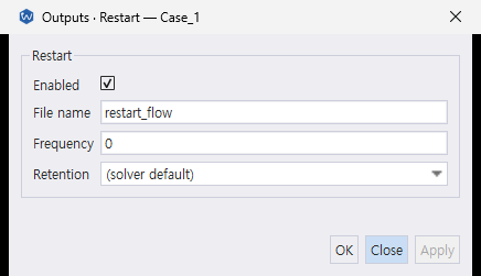
The Desktop exposes the operational restart controls shown above. The contents level in the JSONC example is an advanced CLI setting and is not currently shown in this dialog.

{
  "outputs": {
    "restart": {
      "enabled": true,
      "file_name": "restart_flow",
      "frequency": 100,
      "contents": "full",
      "retention": { "policy": "keep_last", "count": 2 }
    }
  }
}

contents controls how much mesh data is embedded in the .wsol restart. frequency: 0 writes only at the final iteration. Choose the content level and retention policy from the restart workflow you actually need.

contents	What the restart contains	Use when
fields	Solution fields only	The original mesh is always available and you want the smallest restart files.
geometry	Fields, coordinates, and boundary-node sets	You need to remap onto a mesh without reopening the original mesh file.
full (default)	Fields plus connectivity	You need a mesh-file-free restart; this is the safest operational default.

retention.policy is keep_last, keep_all, or milestone:

Policy	What it keeps	When to use it
(no periodic writes; frequency: 0)	Final iteration only	Short or cheap-to-rerun cases where losing all progress on a crash is an acceptable risk. No mid-run write overhead at all.
keep_last + count	The count most recent writes; older ones are pruned as new ones arrive	The default choice for a long run: crash recovery within one frequency interval of progress, bounded disk use.
milestone + milestones	Only the listed iterations, plus the final iteration	You want both crash recovery and permanent snapshots at specific points you’ll want to inspect later (e.g. “did the flow reach its expected transient-to-periodic transition by iteration X?”).

Important

milestone ignores frequency entirely. The solver writes only at the listed milestones (which do not need to be multiples of frequency — any iteration number is allowed) plus the final iteration; no other restart file is ever created, so there is nothing to prune. If you want, say, one checkpoint roughly every second of physical time on a run with a CFL-limited, slowly-drifting Δt, compute approximate target iterations from your expected Δt and list them explicitly — exact alignment with the true Δt at that point in the run isn’t necessary, since these are just recovery points.

{
  "outputs": {
    "restart": {
      "enabled": true,
      "file_name": "restart_flow",
      "retention": {
        "policy": "milestone",
        "milestones": [928505, 1857010, 2785515, 3714020]
      }
    }
  }
}

23.4 volumes

Figure 23.2: A volume-output entry writing the default flow fields in ParaView VTU format. A frequency of zero means final iteration only.

Note

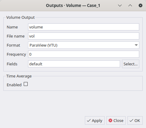
The current source additionally exposes Enabled and Start iteration above the fields shown in this capture. They map to enabled and start_iter in the same output entry.

{
  "outputs": {
    "volumes": [
      {
        "name": "flowfield",
        "file_name": "volume_output",
        "format": "vtu",
        "enabled": true,
        "start_iter": 0,
        "frequency": 100,
        "fields": ["default", "Entropy"],
        "enable_vtm": false,
        "subdivision": -1
      }
    ]
  }
}

format is one of vtu, vtkhdf, tecplot, cgns, or tecplot_binary. These are container names and take no aliases: paraview is not a value, though both vtu and vtkhdf open in ParaView. vtkhdf is the one to reach for on an MPI run: it writes a single HDF5 container across ranks instead of the .pvtu + one .vtu-per-rank split that plain vtu produces.

fields accepts "default" (or omit fields entirely — same thing) plus any individual field names to add on top: ["default", "Entropy", "TotalPressure"]. "default" itself adapts to the physics model you declared in models — Euler gives density/velocity/pressure/temperature/ Mach/Cp, Navier–Stokes adds laminar viscosity and wall distance, RANS adds eddy viscosity and the turbulence variable(s). The old per-model presets ("euler", "ns", "rans") are gone — since the physics model is already declared in models, repeating it in outputs was redundant, and today it’s rejected outright rather than silently accepted.

subdivision renders high-order FR results as subdivided VTK cells; FVM ignores it.

23.5 surfaces and slices

Figure 23.3: A surface-output entry writing pressure, skin friction, wall shear stress, and y+ on the named wall boundary.

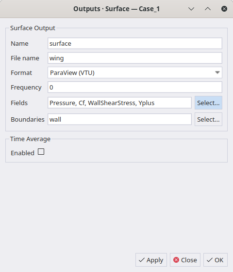
Surface selections use the names of configured boundary objects, not raw mesh marker names. Slice entries use the same common output controls and add plane origin and normal fields; no slice screenshot is included in this set.

{
  "outputs": {
    "surfaces": [{
      "name": "airfoil_surface",
      "file_name": "surface_airfoil",
      "format": "vtu",
      "enabled": true,
      "start_iter": 0,
      "frequency": 100,
      "fields": ["Pressure", "Cp", "Cf", "Yplus"],
      "boundary_names": ["AIRFOIL"]
    }],
    "slices": [{
      "name": "mid_plane",
      "file_name": "slice_mid",
      "format": "vtu",
      "enabled": true,
      "start_iter": 0,
      "frequency": 100,
      "fields": ["Pressure", "Mach"],
      "normal": [0, 0, 1],
      "origin": [0, 0, 0.5]
    }]
  }
}

surfaces carries wall/boundary quantities such as Cf, Yplus, and wall pressure — force-and-moment post-processing territory. It is not what shows flow structures like a vortex street or a shock: for that you need volumes (the full-domain field). In a 2D case in particular, a surfaces entry is just the wall curve — useful for Cf/WSS/wall-pressure plots (which are already covered by a force/pressure monitoring history CSV in most cases), but pointless for animating the flow field itself. Don’t enable surfaces output purely to build a wake/shock animation; enable volumes instead and leave surfaces at frequency: 0 unless you specifically need per-frame wall data.

23.6 Choosing a frequency for volume/surface output

frequency is in solver iterations, not physical time, so the right value depends on what the output is for:

• Quantitative comparison only (final CD/CL, a converged wall-pressure distribution, and so on): frequency: 0 (final iteration only) is enough — there is no reason to pay for intermediate files.

• Animation of an unsteady phenomenon (vortex shedding, a moving shock, transient startup): work backward from how many frames per cycle you want, then convert to an iteration interval:

  frequency ≈ (period of the phenomenon) / (target frames per period) / Δt

  For example, a shedding period T_shed ≈ 0.358 s and a fixed BDF Δt of 1e-3 s gives T_shed / Δt ≈ 358 steps per period; a frequency: 25 yields about 14 frames per period — light enough to keep file counts low over a long run (tens of thousands of steps) while still showing the motion. Wanting a smoother ~25–30 frames per period instead means using a smaller frequency (or, for an explicit run whose Δt is itself CFL-driven and not fixed, recomputing the target iteration interval from the current Δt rather than assuming it stays constant across the run).

Every volume/surface write costs real disk space (a fine 2D mesh’s flow volume file can run a few megabytes each), so before committing to a frequency for a run that will take many hours, multiply out (iterations to run) / frequency × (size of one file) and compare against available disk — it’s a cheap sanity check that avoids discovering you picked too dense an interval after the run is already hours in.

23.7 time_average

Instead of the old statistics block, attach time_average to each output entry individually.

{
  "outputs": {
    "volumes": [{
      "name": "mean_flow",
      "format": "vtu",
      "fields": ["Pressure", "Velocity_x"],
      "time_average": {
        "enabled": true,
        "start_iter": 500,
        "rms": false,
        "fields": ["Pressure", "Velocity_x"]
      }
    }]
  }
}

Time averaging is supported for volumes only. Enabling it on a surface or slice is rejected.

23.8 diagnostics

{
  "outputs": {
    "diagnostics": {
      "state_extrema": { "enabled": true, "frequency": 1 },
      "on_diverge": { "volume_dump": true },
      "fr_reference_compare": { "path": "", "centred": true },
      "dump_linsys": { "enabled": false, "iter": [100, 200], "path": "linsys" }
    }
  }
}

state_extrema records the min/max of every conserved variable (and where it occurred) to solver_state_extrema.csv. Its frequency controls the diagnostic interval. Disable it to avoid the associated GPU reduction and MPI merge.

Diagnostic	Use	Operational note
state_extrema	Locate a nonphysical state before or during divergence.	Costs a GPU reduction and MPI merge at each configured frequency.
on_diverge	Write the volume field at divergence.	volume_dump is the only key: the dump follows the configured volume output rather than taking its own field list.
dump_linsys	Inspect the active linear system at selected outer iterations.	Development or solver-diagnosis tool; do not leave it enabled in normal production runs.
fr_reference_compare	Compare an FR solution against a reference implementation.	Cross-validation only, not ordinary result output.

dump_linsys writes the active solver’s Jacobian and RHS in Matrix Market format. Its iter list accepts at most 16 outer iterations; an empty path uses the run output directory.

dump_linsys is a diagnostic option that dumps the linear system to a file at the specified iterations.

print_inner_iter (dual-time inner-vs-outer row selection, shared between the console and the residual CSVs) lives under monitoring, not here.

FR also doesn’t use a separate fr_dump or fr_force_monitor. It uses the standard volumes[] and monitoring.monitors[]. Use outputs.restart for solution-point snapshots; the former diagnostics.fr_snapshot key was removed. fr_reference_compare is for cross-checking against a reference implementation.

23.9 Setting this from the CLI

{
  "outputs": {
    "surfaces": [{
      "name": "wing_surface",
      "boundary_names": ["wing"],
      "file_name": "wing_surface",
      "format": "vtu",
      "frequency": 1000,
      "fields": ["Pressure", "Cp", "Mach"]
    }]
  }
}

23.10 Rotating-frame energy field

Rothalpy is I = H − U·v in J/kg, where U is grid/frame velocity. It is available in volume, surface, and slice outputs. In rotating DBNS cases it helps compare the relative-frame energy balance.

Surface output requires explicit boundary_names and fields; field bundles such as default are not accepted there. The removed wallvars bundle must be replaced with individual fields such as Cf, WallShearStress, HeatFlux, and Yplus. Wall quantities require DBNS viscous no-slip walls for every selected boundary. Surface CGNS and surface/slice time averaging are rejected. Explicit fields that the physics cannot produce are rejected rather than silently omitted; 2D Helicity is also rejected.