21 Run control and convergence
Iteration limits, convergence criteria, and steady/unsteady time progression
Choose analysis.time and analysis.solver first. Then use this page to set when the run stops, the physical time step (unsteady cases), and the pseudo-time step used to converge a steady solution or an implicit physical step. The GUI Run Control panel and the CLI run_control block write the same settings. Solver schemes and linear solvers are described in Numerical methods.
Physical time Δt advances the simulated clock. Pseudo-time Δτ only helps converge a steady solution or an implicit physical step; it does not advance that clock. run_control.timestep is Δt, while run_control.pseudo_time.timestep is Δτ. A CFL value can control either one, depending on the solver and time scheme below.
21.1 Configure in the GUI
The Desktop Run Control editor opens from the Run Control node of the project outline and writes the same run_control keys the CLI reads. Its three tabs separate the three questions this page answers: Loop sets the stopping limit, Convergence the criteria that may stop a run earlier, and CFL the pseudo-time step.
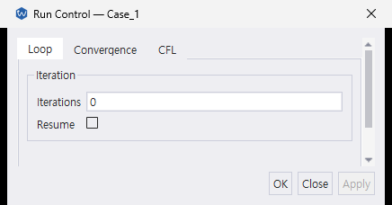
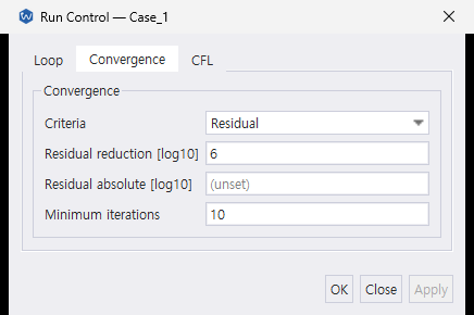
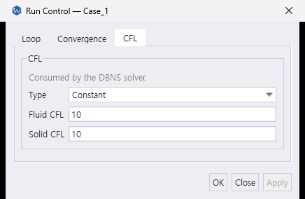
| Tab | GUI control | Input key | What to choose |
|---|---|---|---|
| Loop | Iterations | run_control.iteration |
The outer iteration limit. A steady run stops here unless a convergence criterion stops it first. |
| Loop | Resume | run_control.resume |
Continue from a restart file instead of the initial field. |
| Convergence | Criteria | run_control.convergence.criteria |
residual or monitor. The fields below belong to residual. |
| Convergence | Residual reduction [log10] | run_control.convergence.residual_reduction |
Orders of magnitude the residual must fall from its starting value. |
| Convergence | Residual absolute [log10] | run_control.convergence.residual_absolute |
An absolute floor. An empty field leaves the key unset. |
| Convergence | Minimum iterations | run_control.convergence.min_iter |
Iterations to run before either criterion is tested. |
| CFL | Type | run_control.cfl.type |
constant, schedule, or adaptive. |
| CFL | Fluid CFL | run_control.cfl.fluid.value |
The fluid-zone CFL for constant. |
| CFL | Solid CFL | run_control.cfl.solid.value |
The CHT solid-zone CFL, a fixed value only. |
The CFL tab states that its values are consumed by the DBNS solver; a PBNS case takes its pseudo-time step from pseudo_time instead.
The unsteady keys — timestep, total_time, pseudo_time and timestep_control — are not in this dialog. Write them in JSONC.
21.2 Choose a setup
| Analysis | Physical time and stopping rule | Convergence/step-size controls |
|---|---|---|
| DBNS steady | Set iteration; convergence may stop earlier. |
Set cfl for the pseudo-time step. |
| PBNS steady | Set iteration; convergence may stop earlier. |
Set pseudo_time; tune numerical_method.pbns outer/relaxation controls if needed. cfl does not control PBNS. |
DBNS unsteady, standard |
Set total_time and optionally iteration; whichever limit is reached first stops the run. |
cfl sets the explicit physical Δt unless timestep is supplied. There is no inner loop. |
DBNS unsteady, bdf1/bdf2 |
Set physical timestep and total_time; iteration is a second limit. |
cfl controls inner pseudo-time progress; convergence.inner bounds each physical step’s inner iterations. |
| PBNS unsteady | Use standard (native adaptive-Δt BDF1), initial timestep, and total_time. |
numerical_method.pbns.timestep.cfl_acoustic, .cfl_flow, and .cfl_diffusion limit the evolving physical Δt; pbns.coupling.max_iter/.rho_tol govern the per-step solve. |
FR unsteady, standard |
Set timestep and total_time; optionally use timestep_control to adapt physical Δt. |
Choose the explicit integrator in numerical_method.fr.time_integration. FR has no steady mode. |
FR unsteady, bdf1/bdf2/sdirk3/sdirk4 |
Set physical timestep and total_time. |
pseudo_time controls Δτ; convergence.inner controls the inner solve, with numerical_method.fr.pseudo_scheme. |
Start with the example matching your solver, then change the limits and step size for your case. These are analysis/run_control excerpts, not complete cases; mesh, models, and other required blocks are omitted.
21.2.1 DBNS steady
{
  "analysis": { "solver": "dbns", "time": "steady" },
  "run_control": {
    "iteration": 3000,
    "cfl": { "type": "constant", "fluid": { "value": 10 } },
    "convergence": {
      "criteria": "residual",
      "residual_reduction": 5,
      "min_iter": 10
    }
  }
}
21.2.2 PBNS steady
{
  "analysis": { "solver": "pbns", "time": "steady", "dimension": 3 },
  "run_control": {
    "iteration": 3000,
    "pseudo_time": { "type": "auto", "factor": 1.0 },
    "convergence": {
      "criteria": "residual",
      "residual_reduction": 5,
      "residual_absolute": -15
    }
  }
}
21.2.3 DBNS unsteady: explicit
{
  "analysis": { "solver": "dbns", "time": "unsteady" },
  "run_control": {
    "time_stepping": "standard",
    "cfl": { "type": "constant", "fluid": { "value": 1.0 } },
    "total_time": 0.1
  }
}
21.2.4 DBNS unsteady: dual time
{
  "analysis": { "solver": "dbns", "time": "unsteady" },
  "run_control": {
    "time_stepping": "bdf2",
    "timestep": 1.0e-3,
    "total_time": 0.1,
    "cfl": { "type": "constant", "fluid": { "value": 10 } },
    "convergence": { "inner": { "min_iter": 2, "max_iter": 200 } }
  }
}
21.2.5 PBNS unsteady
{
  "analysis": { "solver": "pbns", "time": "unsteady", "dimension": 3 },
  "numerical_method": {
    "pbns": {
      "timestep": { "cfl_acoustic": 50.0, "cfl_flow": 0.5, "cfl_diffusion": 0.5 },
      "coupling": { "max_iter": 20 }
    }
  },
  "run_control": {
    "time_stepping": "standard",
    "timestep": 1.0e-4,
    "total_time": 0.1
  }
}
21.2.6 FR unsteady: explicit
{
  "analysis": { "solver": "fr", "time": "unsteady" },
  "numerical_method": { "fr": { "time_integration": "rk4" } },
  "run_control": {
    "time_stepping": "standard",
    "timestep": 1.0e-4,
    "total_time": 0.1
  }
}
21.2.7 FR unsteady: dual time
{
  "analysis": { "solver": "fr", "time": "unsteady" },
  "numerical_method": { "fr": { "pseudo_scheme": "tvd_rk3" } },
  "run_control": {
    "time_stepping": "bdf2",
    "timestep": 1.0e-3,
    "total_time": 0.1,
    "pseudo_time": { "type": "cfl", "cfl": 1.0, "beta": 1.0 },
    "convergence": { "inner": { "min_iter": 2, "max_iter": 200 } }
  }
}
21.3 Limits and restart
21.3.1 iteration, total_time
iteration is the upper bound on outer iterations/physical steps, not the inner iterations of one dual-time step. max_iter is a compatibility alias; use iteration in new files. In steady analysis, convergence may stop the run before this limit. In unsteady analysis, iteration and total_time (physical seconds) are independent limits: the first reached stops the run. If you only care about elapsed physical time, set total_time explicitly; the unsteady default is 50 s and the iteration default is 999999.
For fixed Δt, estimate the required step count as total_time / timestep. With adaptive Δt (PBNS or FR PI control), inspect the physical-time column in the run output instead of assuming a fixed count.
21.3.2 resume
Controls whether initialization.type=restart also restores run state.
| Value | Behavior |
|---|---|
false (default) |
Warm start: use the saved flow field as a new initial condition; reset the iteration counter, physical time, and time history. Use this when changing from steady to unsteady analysis. |
true |
Resume: restore the iteration counter, physical time, BDF history, and saved run state (including residual baseline and adaptive CFL state where applicable). Use this to continue an interrupted run. |
21.4 CFL
cfl is DBNS only. It controls pseudo-time progress in steady and dual-time calculations; with standard unsteady stepping it controls the explicit physical Δt instead. Start with a constant value. If convergence is smooth but slow, try a schedule or adaptive control; if residuals oscillate or states become non-physical, reduce the CFL. For a CHT solid zone, set cfl.solid.value separately (fixed value only).
This block used to live at numerical_method.dbns.cfl_control. That path is no longer accepted and parsing fails if it is still present. Along with the move, type: scheduled_ramp was renamed to schedule.
type |
Fields used |
|---|---|
constant |
fluid.value |
schedule (alias ramp) |
fluid.schedule[] — iter, value, ramp_iters |
adaptive |
fluid.adaptive.* — start, min, max, factor_down, factor_up, acceptable_linear_residual, start_iter, per_point |
adaptive cannot be used with standard unsteady stepping.
21.4.1 CFL means something different for implicit and explicit schemes
The role of cfl depends entirely on run_control.time_stepping (see Unsteady physical time below), and this is the single most common point of confusion when setting up an unsteady DBNS case:
bdf1/bdf2(implicit dual-time):run_control.timestepfixes the physical Δt directly and dimensionally (e.g.1.0e-3seconds).cflonly controls how aggressively the inner pseudo-time iterations converge the nonlinear system at each physical step — it has no effect on the physical time step. Choosetimestepfor the temporal accuracy you need, then check that each physical step’s inner residual converges withinconvergence.inner.max_iter. An implicit scheme does not guarantee a stable or accurate result for an arbitrarily large step.standard(explicit): there is no pseudo-time loop, socfldirectly determines the physical Δt at every step:dt = cfl · h / (|u| + a), evaluated per cell and reduced to a single global Δt applied to the whole domain (this is global time stepping — required for time accuracy; the per-cell local time stepping used to accelerate steady convergence would desynchronize the physical time across the domain and is not valid here). Because this Δt is recomputed from the current mesh and flow state at every step, it also drifts slightly as the solution develops.You can set
run_control.timestepdirectly instead, but then you must check its stability limit against the smallest cells and local wave speeds. Starting with a modest CFL is usually easier.TipSmall near-wall cells can force a very small global Δt. Check the reported Δt and estimated number of steps before committing to a long explicit run.
21.4.2 schedule
iter is the outer iteration at which that breakpoint takes effect, and ramp_iters is the transition length from the previous value. null or 0 means an immediate jump; the first entry’s ramp_iters is ignored.
{
  "run_control": {
    "cfl": {
      "type": "schedule",
      "fluid": {
        "schedule": [
          { "iter": 0,   "value": 1,  "ramp_iters": null },
          { "iter": 100, "value": 5,  "ramp_iters": 20 },
          { "iter": 500, "value": 20, "ramp_iters": 10 }
        ]
      }
    }
  }
}
21.4.3 adaptive
adaptive adjusts the CFL from what the previous iteration already told you: the linear solver’s relative residual, each point’s implicit under-relaxation, and the trend of the nonlinear residual. It is a CFL policy — unlike HANIM it never rejects a trial state, restores Uⁿ, or retries an iteration.
Set run_control.cfl.type to adaptive. The keys below are inside run_control.cfl.fluid.adaptive.
| Key | Default | Meaning |
|---|---|---|
start |
5.0 |
Initial CFL; must lie in [min, max]. The per-point field is seeded uniformly with it. |
min |
5.0 |
Band floor, and the target of a reset. |
max |
100.0 |
Band ceiling. |
factor_down |
0.1 |
Multiplier applied when a point is strongly under-relaxed or the linear solve missed its target. |
factor_up |
1.2 |
Multiplier applied when the point took the full update and the linear solve met its target. |
acceptable_linear_residual |
0.1 |
Linear-residual target for the controller (see below). |
start_iter |
0 |
No raise or cut before this outer iteration. |
per_point |
true |
Per-point CFL field; false drives one scalar CFL instead. |
{
  "run_control": {
    "cfl": {
      "type": "adaptive",
      "fluid": { "adaptive": { "start": 5.0, "min": 5.0, "max": 100.0 } }
    }
  }
}
How a step is decided. The controller first forms one target from your two tolerances, linTol = max(acceptable_linear_residual, linear_solver.error), and compares it against the worst relative linear residual of the previous iteration (mean flow and turbulence):
- below
linTol→ the point may be raised, - above
1.2 · linTol→ the point is cut, - in between → held. The 20 % dead band exists to stop the CFL flip-flopping.
A linear residual above 0.99, or a nonlinear residual that has risen more than two orders across the last 100 iterations, resets every point to min.
Each point then applies its own under-relaxation UR = min(UR_flow, UR_turb), the factor the implicit update had to use to keep the state physical: UR < 0.1 multiplies by factor_down, a full UR = 1 with a healthy linear solve multiplies by factor_up, and anything between holds. With per_point: true this runs on the CFL field, so stiff cells (a shock, a degenerate wall cell) hold or drop while the rest of the mesh climbs; the scalar CFL you see in the console and in restarts is the minimum over points. With per_point: false the same three-way rule is driven by the global minimum UR instead.
max is part of the design, not a safety net you should remove. The controller only sees the linear solver, so if the linear solve keeps succeeding it will keep raising the CFL until the state itself goes non-physical. Keeping the default ceiling of 100 is what makes the policy stable; raising it to 1e4 on a 2-D airfoil case produced a CFL sawtooth and non-physical states that had to be rolled back, with a worse residual than the capped run.
HANIM is selected separately through numerical_method.dbns.nonlinear_control.method: "hanim" with time_integration: "jfnk". By default HANIM has no startup phase and does not use run_control.cfl at all — it starts from nonlinear_control.cfl_start on the first iteration. If the deck sets jfnk.startup_iter or startup_residual_reduction, adaptive (or any other policy) drives that startup and HANIM inherits the CFL when it activates, taking the minimum over points but never below cfl_start.
Do not use adaptive with time_stepping: "standard" unsteady analysis. The validator rejects that combination. run_control.cfl is DBNS-only; PBNS and FR use their solver-specific pseudo-time controls.
numerical_method.dbns.cfl and cfl_solid were removed. Set DBNS CFL only under run_control.cfl.
21.5 pseudo_time
The pseudo-Δτ policy. Two solvers consume it:
- PBNS steady — the false-transient step used to approach the steady solution (
analysis.solver=pbnswithanalysis.time=steady). - FR dual time — the inner-iteration Δτ, whenever
time_steppingis something other thanstandard.
PBNS unsteady does not consume this block. It uses numerical_method.pbns.{cfl_acoustic,cfl_flow,cfl_diffusion} to limit an adaptive physical Δt. Start PBNS steady with auto; if it is too aggressive, lower factor. Use timestep when a measured pseudo-time scale is known, or cfl when the mesh and local flow should determine Δτ.
{
  "run_control": {
    "pseudo_time": {
      "type": "auto",
      "factor": 1.0,
      "timestep": 1.0e-3,
      "cfl": 5.0,
      "beta": 1.0,
      "adaptive": {
        "controller": "local_pi",
        "atol": 1.0e-5,
        "pi_alpha": 0.7,
        "pi_beta": 0.4,
        "safety_factor": 0.8,
        "factor_down": 0.98,
        "factor_up": 1.01,
        "max_factor": 2.0
      }
    }
  }
}
type |
Active fields | Meaning |
|---|---|---|
auto (default) |
factor |
Fixed Δτ = factor · L/U, determined at run start. L comes from reference.length_moment; U uses the initial/farfield/inlet speed and reference.velocity, with sound speed as the compressible zero-speed fallback. Constant-density cases need a nonzero velocity reference. Lower factor if the steady solve is unstable. |
timestep |
timestep |
Uniform pseudo-time Δτ in seconds; this is not the physical run_control.timestep. |
cfl |
cfl, beta |
Local Δτ = cfl · h / (\|u\| + β·a); β = 1 includes the acoustic speed, while a smaller positive β moves toward a convective scale. FR additionally accounts for polynomial order. |
adaptive is an FR-only embedded-error controller for the pseudo step; it needs numerical_method.fr.pseudo_scheme to be rk34 or rk45. It spells its gains exactly like timestep_control below, because they are the same kind of controller applied to a different step.
pseudo_time.adaptive key |
Effect (FR dual time only) |
|---|---|
controller |
none (default) or local_pi; enable the latter only with an embedded rk34/rk45 pseudo scheme. |
atol |
Absolute error scale for the embedded estimate. |
pi_alpha, pi_beta |
PI response to current and previous error. Start with defaults (0.7, 0.4). |
safety_factor |
Multiplies the proposed next Δτ; default 0.8. |
factor_down, factor_up |
Bound how much Δτ can shrink or grow per step; defaults 0.98, 1.01. |
max_factor |
Caps the initial Δτ multiplier; default 3.0. |
This key lives at run_control.pseudo_time, not inside a solver’s numerical_method block — it moved here for the same reason cfl did. The three are not exclusive but consumed by different solvers: cfl drives DBNS, pseudo_time drives PBNS steady and FR dual time, and timestep_control drives FR explicit.
21.6 timestep_control
The physical-Δt policy: an embedded-error PI controller that resizes Δt every step. FR explicit only, and only with numerical_method.fr.time_integration set to rk34 or rk45. Leave controller: "none" (the default) for a fixed run_control.timestep. Do not combine PI control with FR entropy filtering or dual time; the solver rejects those combinations.
{
  "run_control": {
    "timestep_control": {
      "controller": "pi",
      "atol": 1.0e-6,
      "rtol": 1.0e-6,
      "error_norm": "l2",
      "pi_alpha": 0.58,
      "pi_beta": 0.42,
      "safety_factor": 0.8,
      "factor_down": 0.3,
      "factor_up": 2.5,
      "min": 1.0e-12,
      "max": 1.0e2
    }
  }
}| Key | Meaning |
|---|---|
controller |
none (default) or pi |
atol, rtol |
Absolute/relative error tolerances driving the step-size estimate; tighten them for a more accurate, usually slower run. Defaults are 1e-6 each. |
error_norm |
l2 or uniform |
pi_alpha, pi_beta |
PI-controller gains; defaults 0.58, 0.42 |
safety_factor |
Multiplier on the proposed step; default 0.8 |
factor_down, factor_up |
Limits on the change per step; defaults 0.3, 2.5 |
min, max |
Absolute bounds on physical Δt; below min the run fails. Defaults 1e-12, 1e2 s. |
21.7 Convergence criteria
For a steady run, convergence can end the outer loop before iteration. For DBNS/FR dual time, it can end each inner solve before convergence.inner.max_iter. Standard unsteady runs advance until total_time or iteration instead. In DBNS residual convergence, the relative and absolute tests form an OR: whichever threshold is met first ends that loop. FR dual time uses inner.residual_tol (or the iteration cap when that tolerance is zero). criteria: "monitor" selects a monitor-based steady stopping rule instead.
21.7.1 residual
The default criteria. For DBNS, residual_reduction is the log10 order-of-magnitude drop relative to a baseline. PBNS steady is different: it compares its already-scaled pressure-based residual directly with 10^-residual_reduction, without dividing by an initial residual. Use the pressure-based residual to judge PBNS steady convergence; the absolute threshold is usually a deep safety net (-15 in the reference deck). min_iter delays the steady outer-loop test.
{
  "run_control": {
    "convergence": {
      "criteria": "residual",
      "residual_reduction": 5,
      "min_iter": 10,
      "inner": { "min_iter": 2, "max_iter": 200 }
    }
  }
}| Key | Meaning |
|---|---|
criteria |
residual (default) or monitor; picks which steady stopping test to use. |
residual_reduction |
Default 5. DBNS: stop after this many orders of reduction from the loop baseline. PBNS steady: require its scaled pressure-based residual to be at most 10^-N. |
residual_absolute |
Stop when log10\|R\| reaches this value; default -8 for steady and -14 for dual-time inner solves. DBNS uses L2 RMS; PBNS uses a weighted RMS, so do not compare the two values directly. |
min_iter |
Outer loop only: don’t evaluate convergence before this many iterations. Not inherited by inner. |
inner.min_iter / inner.max_iter |
Minimum/maximum pseudo-time iterations per physical step for DBNS/FR dual time; defaults 2/200. Replace the old top-level inner_iter with inner.max_iter. If the cap is reached while the inner residual is still high, increase it or ease the physical timestep. |
inner.residual_tol / inner.residual_norm |
FR inner residual gate. 0 (default) uses the iteration cap without this tolerance test; residual_norm is l2 or uniform. |
The DBNS relative-residual baseline depends on the loop:
| Loop | Baseline for residual_reduction |
|---|---|
| Steady outer | The maximum residual over the first 5 samples (a warm-up peak, more representative than iteration 1) |
| Dual-time inner | The residual at the start of that physical step |
residual_absolute’s default follows the same DBNS split: for an inner solve the absolute check is only an escape hatch for a step that enters already near machine-zero residual — the steady default (-8) would fire on nearly every step there, so the inner default is a much deeper -14.
PBNS unsteady has a native BDF1 outer solve per physical step. Its per-step controls are numerical_method.pbns.max_outer and outer_tol, not the DBNS/FR dual-time convergence.inner settings.
21.7.2 monitor
Stop once a named monitor’s value has settled, instead of waiting on the residual — useful when the residual sits on a floor without dropping further while the quantity you actually care about (a force coefficient, say) has already stopped changing.
{
  "run_control": {
    "convergence": {
      "criteria": "monitor",
      "monitor": {
        "fields": ["CFx", "CFy"],
        "eps": 1.0e-5,
        "window": 100
      }
    }
  }
}
monitor.fields lists the monitor names to test, window is the number of recent outer iterations (default 100), and eps is the tolerance (default 1e-5). For each listed field:
(max − min) / max(|max|, 1.0) < epsso a coefficient with |value| ≤ 1 is judged on an absolute basis (the default eps = 1e-5 is roughly 0.1 drag/lift count), while a larger physical quantity is judged relatively. Every listed field has to settle — it’s an AND, not an OR. fields entries must match a monitoring.monitors[] block’s name (or <name>.<boundary> for a per-boundary scalar); an unknown name is rejected at validation time, not silently ignored at run time. The window also has to fill up within this run before it can trigger, so resuming a run doesn’t stop it immediately just because the first few post-restart samples happen to look flat.
21.8 Unsteady physical time
Set analysis.time: "unsteady" before choosing time_stepping. The physical clock advances by Δt until total_time or iteration is reached.
{
  "analysis": { "time": "unsteady" },
  "run_control": {
    "time_stepping": "bdf2",
    "timestep": 1.0e-3,
    "total_time": 3.0
  }
}
time_stepping |
DBNS | PBNS | FR |
|---|---|---|---|
standard (default) |
Explicit; CFL-derived physical Δt, or user-supplied timestep. |
Native first-order BDF with adaptive Δt and per-step outer solve. | Explicit integrator selected by numerical_method.fr.time_integration; fixed timestep or adaptive timestep_control. |
bdf1 |
First-order dual time. | Alias of standard; the same native BDF1 path. |
First-order dual time. |
bdf2 |
Second-order dual time. | Rejected: not implemented. | Second-order dual time, supported since September 2026. First step and steps after Δt changes start with BDF1; a resumed run can restore BDF2 history from its restart file. |
sdirk3, sdirk4 |
Not supported. | Not supported. | Three-stage, third-/fourth-order dual-time schemes respectively. |
21.8.1 timestep and total_time
timestep is the physical initial or fixed Δt in seconds, depending on solver:
- DBNS
standard: omit it to derive Δt fromrun_control.cfl; if supplied, verify explicit stability yourself. DBNS dual time: it is the fixed Δt; choose it for time accuracy, then ensure the inner solve converges. - PBNS unsteady: it is the initial Δt, not a fixed step. The solver changes it according to its acoustic, flow, and diffusion CFL limits and per-step solve behavior. Check reported physical time and actual Δt when comparing results. PBNS has no fixed-Δt mode.
- FR
standard: it is the fixed starting Δt. Withtimestep_control.controller: "pi", the embedded error estimate changes it each step. FR dual time: it is the physical Δt;pseudo_timesets the separate inner Δτ.
total_time sets the stopping time in seconds. State it explicitly in an unsteady deck; if omitted, the default is 50 s. iteration is also active, and whichever limit is reached first ends the run. For DBNS/FR dual time, the per-step inner limit belongs to convergence.inner.max_iter.
These time-progression keys are not used when analysis.time=steady.
run_control.convergence (this page) and outputs.restart are independent axes — one governs when the run stops, the other governs what gets saved along the way and whether you can resume a crashed run. See File output for restart frequency and retention policy.
21.9 Controlling a running job
For graceful stop signals, scheduled stop/dump via wake.control.json, and gRPC runtime control, see Controlling a running job.
21.10 Restart numbering and FP32 convergence
Iteration-number controls (iteration, min_iter, start_iter, startup_iter, freeze iterations, and CFL schedule iter) use absolute outer-iteration numbers. Resuming does not restart these counters.
The wake_<2|3>d_fp32 build uses float arithmetic on the residual path and may reach a relative residual floor around 1e-7. This is not a universal stopping threshold: check the monitored physical quantities and choose criteria: "monitor" when appropriate. Use _fp64 for precision comparisons and _mixed for double-precision residual arithmetic with FP32 linear solves.